geointerpo¶

Point data in. Smooth interpolated raster out.
18 methods · live weather & air-quality APIs · uncertainty quantification · interactive maps.

Get Started Browse Methods GitHub

Why geointerpo?¶

One API, 18 methods

Every algorithm shares .fit() → .predict(). Swap method= to compare IDW, Kriging, Cokriging, SGS, GP, and 12 more without changing any other code.

Browse methods
Smart boundaries

Pass a place name, a file, or a bbox. The pipeline geocodes it, derives the grid, and clips the output automatically.

Boundary guide
Live data, zero setup

Pull real weather and air quality data from Meteostat, OpenAQ, Open-Meteo, and NASA POWER — no API keys needed. ERA5 reanalysis via CDS API.

Data sources
Uncertainty quantification

Kriging variance surfaces, GP posterior std, RF bootstrap intervals, and conformal prediction (MAPIE) — every method can now express how sure it is.

Uncertainty guide
Interactive maps

result.plot_interactive() renders a zoomable map with plotly or leafmap — no static PNG, no extra code.

Visualization guide
Auto-ranked cross-validation

Spatial k-fold or leave-one-out CV runs automatically. result.best_method() and result.rank_methods() tell you which algorithm won.

Pipeline reference
Export anywhere

Save to GeoTIFF, NetCDF, or PNG. Every output carries CRS metadata and is ready for QGIS, ArcGIS, or further analysis.

Examples
50–200× faster IDW

KD-tree vectorized IDW replaces the old per-point loop — identical results, dramatically less waiting on large grids.

What's new in v0.2

Quickstart¶

Three linesUncertaintyCokriging / SGSSpatial CVOffline demo

from geointerpo import Pipeline

result = Pipeline(
    data="stations.csv",
    boundary="Calgary, Alberta, Canada",
    method=["idw", "kriging", "spline"],
    resolution="5km",   # ← km strings now supported
).run()

result.plot()               # side-by-side matplotlib comparison
result.plot_interactive()   # zoomable plotly map
result.best_method()        # → "kriging"
result.rank_methods()       # ranked DataFrame
result.save("outputs/")     # GeoTIFF + PNG + metrics CSV

from geointerpo.interpolators import KrigingInterpolator, MLInterpolator

# Kriging: mean + variance surface
model = KrigingInterpolator().fit(gdf)
mean_da, var_da = model.predict_with_variance(bbox, resolution=0.1)

# RF: bootstrap prediction interval
model = MLInterpolator(method="rf").fit(gdf)
mean, lower, upper = model.predict_with_uncertainty(bbox, alpha=0.1)

# Cokriging with elevation as secondary variable
from geointerpo.interpolators import CokrigingInterpolator

model = CokrigingInterpolator(
    secondary_col="elevation",
    secondary_fn=dem_lookup_fn,   # callable(xs_utm, ys_utm) → elevations
).fit(gdf_with_elevation)
grid = model.predict(bbox, resolution=0.1)

# Sequential Gaussian Simulation — stochastic realizations
from geointerpo.interpolators import SGSInterpolator

model = SGSInterpolator(n_realizations=100).fit(gdf)
mean_da, std_da = model.predict_with_std(bbox)
all_realizations = model.realize(bbox)  # (100, n_lat, n_lon) DataArray

from geointerpo.validation.metrics import spatial_cv
from geointerpo.interpolators import IDWInterpolator

model = IDWInterpolator(power=2)
# LOO with 50 km buffer — removes autocorrelation leakage
result = spatial_cv(model, gdf, strategy="loo", buffer_km=50)
print(result["rmse"], result["r"])

result = Pipeline(
    data="sample",
    variable="temperature",
    boundary=(-114.5, 50.8, -113.8, 51.3),
    method=["idw", "kriging"],
    resolution="2km",
).run()

No data? No problem.

Use data="sample" for a built-in synthetic dataset — no network, no API keys, runs in seconds.

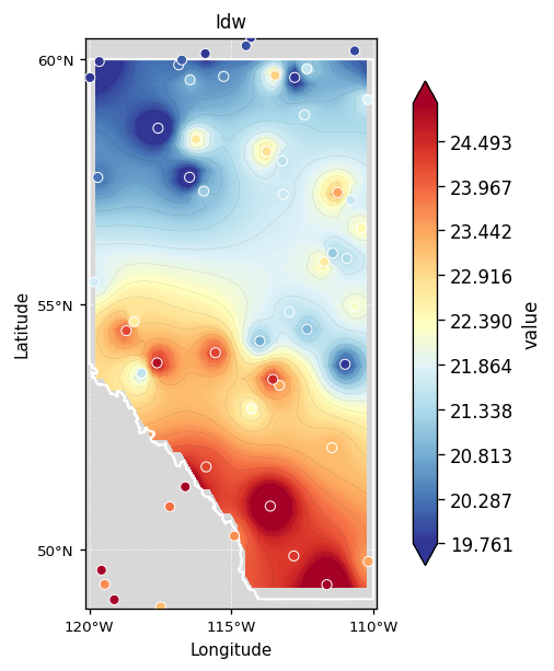
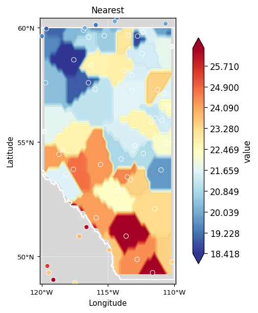
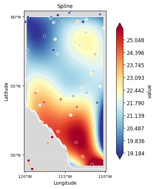
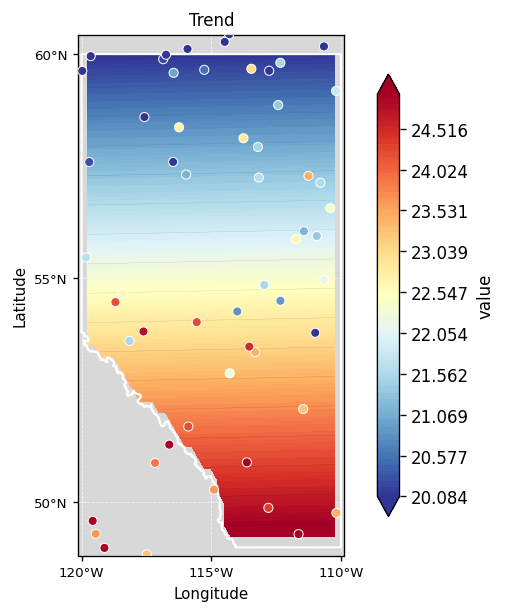
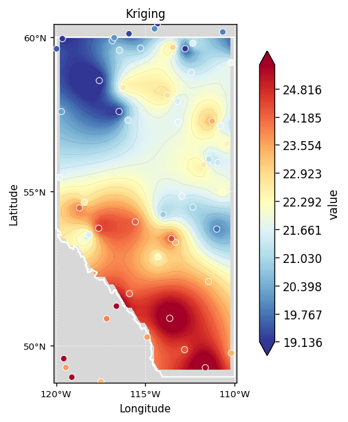
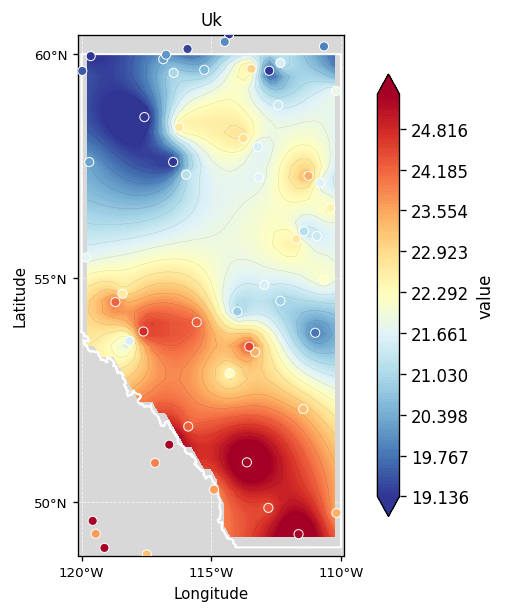
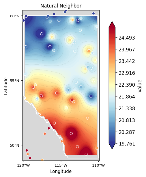
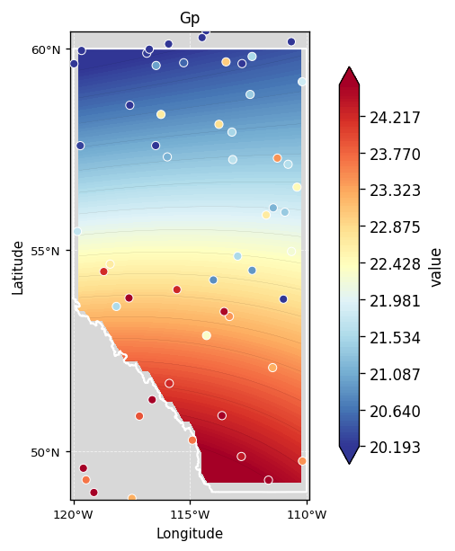
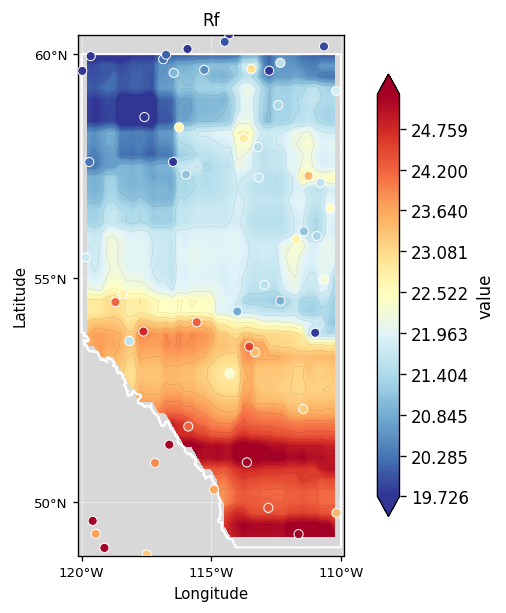
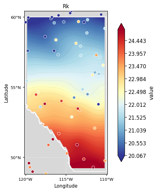
Methods at a glance¶

All outputs below use the same 60 weather stations over Alberta, Canada.

Distance-based¶

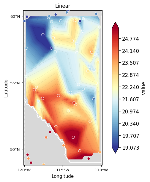
Spline & Trend¶

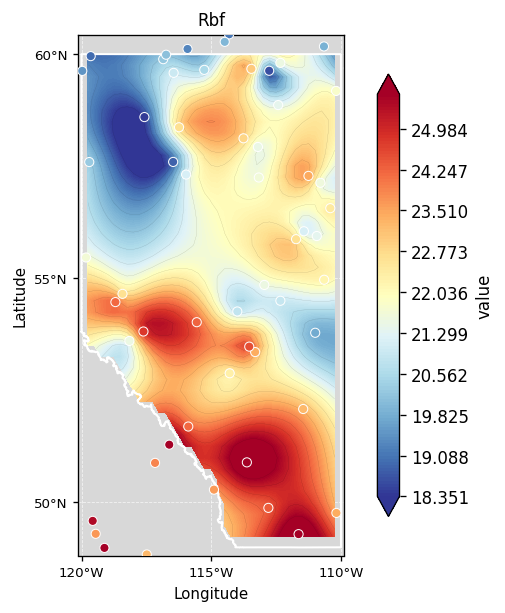
Geostatistical¶

Machine Learning¶

Full method reference with all 18 canonical methods

Install¶

RecommendedCore onlyAdvanced geostatistics (cokriging + SGS)From source

pip install "geointerpo[full]"

pip install geointerpo

pip install "geointerpo[full,geostat]"

git clone https://github.com/homayounrezaie/geointerpo
cd geointerpo && pip install -e ".[full,geostat]"

Full install guide with all extras